Week #3 in MATH 1420

For the students in my online calculus class, here is a guide to events and assignments in the coming week.

Monday, January 30, 2017

1. A trivia question will be posted on Blackboard. (Subscribe to that thread so you get an email as soon as it is posted!)
2. Take Mini-exam 2.
3. Worksheet 1.5 is due by 3 pm.
4. Read/watch Lecture 1.6 on the formal definitions of the limit and the derivative.
5. Begin Worksheet 1.6.

Tuesday, January 31, 2017

1. Read OpenStax section 2.5.
2. Finish Worksheet 1.6.

Open office hours (for ANY math student in any class!) are being offered by me, from 2 to 3:30 at the BSM (Baptist Student Ministry) building on campus, just west of the parking garage.  Drop by!

Wednesday, February 1, 2017

1. Worksheet 1.6 is due by 3 pm.
2. Read/watch Lecture 1.7 on The IRC of Power Functions
3. Begin Worksheet 1.7.

Thursday, February 2, 2017

1. A trivia question will be posted on Blackboard.
2. Read OpenStax sections 3.1 and 3.2.
3. Finish Worksheet 1.7.

Friday, February 3, 2017

1. Worksheet 1.7 is due by 3 pm.
2. Read/watch Lecture 1.8 on The IRC of Trig Functions
3. Begin Worksheet 1.8.

Saturday, February 4, 2017

1. Review OpenStax sections 3.3 and 3.5.
2. Finish Worksheet 1.8.

Monday's Mini-exam 3 (February 6) will be over lectures 1.5-1.8. A total score of at least 20 points on homework is required prior to this mini-exam.  (The first exam is February 13!)

That Number e

One of the more interesting results from limits as x goes to infinity, is the limit of (1+1/x)^x as x goes to infinity.  This limit, introduced by Leonhard Euler, came out of the consideration of exponential functions. (It shows up in finance when interest is compounded.)

As x goes to infinity, 1/x goes to zero.  One might then be tempted to think that (1+1/x)^x goes to 1.  It does not.  The exponent is also going to infinity and so as the expression 1+1/x goes to 1, the expression (1+1/x)^x  stays between 2 and 3.  Here, using the variable n instead of x, is a table of values of (1+1/n)^n as n gets large.

Mathematicians have given this limit a name, defining the constant e to be this limit.

See this Wikipedia webpage on this interesting constant!  The constant e is much more important in mathematics than pi!

Here is e to 100 decimal digits, compliments of WolframAlpha.

2.718281828459045235360287471352662497757247093699959574966967627724076630353547594571382178525166427

What are the strangest constants in mathematics?  Surely the top three are e, pi and i.  At the end of the first part of this course, we will ask the question, What is e^{pi i}? If we combine these three strange constants we get a very simple answer... but that is later.

1.5, Limits and infinity

Today we look at limits involving infinity.  In the first half, we look at the meaning of the input variable, x going to infinity.  In the second half, we examine the meaning of the output variable, y, going to infinity.

Limits as x goes to infinity

Infinity is a mathematical concept, not a number. In this class, we will view (positive) infinity as "larger than any real number" or "beyond all positive real numbers." The limit of f(x), as x goes to infinity, is the value that f(x) approaches, as x grows beyond bound.

For example, consider the rational function f(x) = (4x^2+5x-1)/(3x^2-7x).  What is the limit of f(x) as x goes to infinity.  Consider plugging in big numbers like x equals one billion (1,000,000,000). Here is f(1,000,000,000).

From this computation, it appears that the limit of this function, as x goes to a billion, 1.3333... .

We can build up some intuition about this.  As x gets large, 4x^2 begins to dominate the numerator.  If, for example, x is a billion then x^2 is a billion billion, much larger than 5x which is a mere five billion. So, intuitively, one might argue that only the higher power sof x matter.  If so then we could argue that

Solving limits by algebra

A fundamental example (and major result that we need) is the limit, as x goes to infinity, of 1/x.

As x grows beyond bound, passing a million, billion, ... googol (10^100), ..., googleplex (10^googol), ... and so on, the quantity 1/x becomes smaller and smaller, approaching zero.  If x = 10^n, that is, if x in decimal notation is a 1 followed by n zeroes, then 1/x = 10^(-n), so 1/x, in decimal notation, is a decimal point followed by n-1 zeroes and then a 1.

We summarize this by saying that the limit, as x goes to infinity, of 1/x is 0.

This limit is useful in algebraically simplifying other limits.

For example we could reconsider the function f(x) = (4x^2+5x-1)/(3x^2-7x) mentioned above. Multiplying both numerator and denominator by 1/x^2, we can rewrite the rational function as

(This algebra is correct as long as x is not zero.  Since we are trying to compute that limit as x gets very large, we clearly do not have to concern ourselves with x being zero!)

Since 1/x goes to zero as x goes to infinity, then expressions like 5/x or 1/x^2 or 7/x will go to zero also.  So our limit can be algebraically manipulated as follows:

Limits and vertical asymptotes

Consider the graph, below, of a rational function.  The function is drawn in blue. A vertical asymptote, x = -3,  is drawn in red and a horizontal asymptote, y = 1, is drawn in green.

In this case, as x approaches -3 from the left, the y values shoot up beyond bound. So here we have infinity as a limit!  The output is growing beyond bound!

On the other hand, as x approaches -3 from the right, the y values shoot down out of sight, dropping below every real number.  In this case we say negative infinity is the limit.  Our notation for this would be

The green horizontal asymptote tells us what happens as x goes off to the right, beyond all positive real x-values and also tells us what happens as x goes off to the left, beyond all negative x values. In either case, y is approaching 1 and so our limit is 1.

The vertical asymptotes give us limits of infinity while the horizontal asymptotes describe y values as x goes to infinity.

Resources

Infinite limits are covered in section 2.2 of the OpenStax textbook.

The Mathematical Idea of Conjugate

The simple factoring

A^2 – B^2=(A + B)(A – B)

has lots of applications. The fact that a "difference of squares" factors into a sum times a difference –note the use of three different basic operations! – means that we can often manipulate square roots using this formula.

For example, the cosine of 75 degrees is (using sum of angle formulas) exactly equal to

cos(5 pi/12) = 1/(sqrt(6)+sqrt(2)).

If we don't like the square roots in the denominator, we can multiply both numerator and denominator by (sqrt(6)-sqrt(2)) and the denominator becomes

(sqrt(6))^2-(sqrt(2))^2 = 4.

So another form for the cosine of 75 degrees is

cos(5 pi/12) = (sqrt(6)-sqrt(2))/4.

This is sometimes useful in trying to compute limits.  For example, suppose we seek the limit of

f(x) = (x-4)/(sqrt(x)-2)

as x approaches 4.  If we attempt to substitute in x=4 we simply get an expression which is undefined. But is we multiply numerator and denominator by (sqrt(x)+2), then we get

f(x) = (x-4)(sqrt(x)+2)/(x-4)

which (except at x=4) is equal to

g(x) = sqrt(x)+2.

The limit then, of g(x), as x approaches 4, is equal to g(4) = sqrt(4)+2=2+2=4.  Since g(x) and f(x) agree everywhere except at x=4, they have the same limit there.

Given an expression A+B or A-B, we often speak of the other factor, A-B or A+B, as the conjugate. To simplify the expression f(x) = (x-4)/(sqrt(x)-2), we multiplied by the conjugate of the denominator.

This is especially useful in working with complex numbers. The conjugate of a complex number 

z = a+bi

(where a and b are real numbers) is

z = a–bi.

If we divide one complex number by another, say divide 3+4i by 1-i, we can multiply numerator and denominator by the conjugate of 1-i, that is, multiply by 1+i.

(3+4i)/(1-i) = [(3+4i)(1+i)]/[(1-i)(1+i)].

The denominator will now simplify to 1-i^2 = 2.  So the fraction becomes

(3+4i)/(1-i) = (-1+7i)/2.

The idea of a conjugate appears in the limit of (1-cos x)/x as x approaches zero.  This important limit, used in developing the derivative of the sine function and cosine functions, can be rewritten by multiplying numerator and denominator by the "conjugate" 1+cos x. If we are willing to rewrite 1-cos^2 x as sin^2 x using the trig version of the Pythagorean Theorem, then we have

Once we have this expression, we can recall that the limit of sin x/x is 1 and so

The identity

A^2 – B^2=(A + B)(A – B)

will show up any many areas of mathematics!  Be alert for opportunities to use it!

1.4, Limit laws and continuity

Basic Limit Laws

The concept of the limit was originally developed to analyze behavior near a point where a function is really undefined.  In order to do this, we need some basic ideas about how limits work in routine situations.

For example, if we look at the limit, as x approaches 2, of the function

f(x) = 3x/(x^2+4) 

we should not be surprised to discover that 3x must approach 6 and x^2+4 must approach 8 and so the function approaches 6/8 = 3/4.  We do not need a calculator to argue this.

There are, then, some "obvious" limit laws.  They are described in the OpenStax textbook in section 2.3. (See the box there with 7 different identified laws!) The limit of a sum is the sum of the limits; the limit of a difference is the difference of the limits, etc.  Do NOT memorize these limit law, but merely recognize that the limit acts as you would expect!

We might summarize some of these laws by saying that, except for cases where the denominator is zero, the limit of a polynomial or rational function is "what we would expect" -- just plug the value in!  So the limit of

f(x) = 3x/(x^2+4) 

as x approaches 2 is just f(2) = 3/4.

Computing limits algebraically

If a function is not continuous at a particular point because the graph has a hole there, we can use algebra to remove the gap in the graph and then evaluate the limit by substitution.
For example the following are graphs of two functions.

The first graph is the the graph of f(t)=(t^2+2t-3)/(t^2-1).

The second graph is the graph of g(t) = (t+3)/(t+1).

What is the difference? The first graph has a removable singularity at t=1. Since limit computations only involve questions near a t-value, these two functions have the same limit as t approaches one.
So if we are asked to compute the limit at 1 of the first function, we use algebra to turn it into the second function (near t equal 1 but not at t=1.)  Here are the algebra computations:

The Squeeze Theorem

The "squeeze theorem" says that if a function g(x) is "squeezed" between two functions h(x) and f(x), so that f(x) < g(x) < h(x), and yet, at the place where x=a, the limit of the bottom function f(x) and the top function h(x) are the same, then the function g(x) must have the same limit.

(Download OpenStax materials for free at 

http://cnx.org/contents/8b89d172-2927-466f-8661-01abc7ccdba4@2.37.)

We will find numerous uses for this....

A trig limit

The squeeze theorem is useful finding a very important limit in trigonometry.  Note, from the geometry of the circle, that if the angle theta is close to zero then theta is between the sine of theta and the tangent of theta.

Continuity

A function f(x) is continuous at x=a if the limit of f(x) as x approaches a is equal to f(a).  This means that the limit is what we might expect, that the limit can be found by simply substituting the value a into the function.

Our algebra strategy, above, was to replace a function like  f(t)=(t^2+2t-3)/(t^2-1) by a function g(t) = (t+3)/(t+1) which is continuous at the desired value a. (Here a=1.) Once we have a continuous function, computing limits is easy!

The area of a circle

One early use of limits was in finding the area of a circle.  a nice short explanation of that can be found here. 

1.3, Limits and the IRC

The instantaneous rate of change concept has an inherent difficulty.
It takes the idea of the average rate of change, the slope a secant line between two points and attempts to identify a tangent line hitting the curve at a single point.

Limits and the Instantaneous Rate of Change

A single point does not define a line but we don't let that bother us since we are guided to this tangent line by the secant lines.  Geometrically and algebraically we can often visualize this tangent line as the end result of a sequence of secant lines.

But to be precise and careful about the IRC, we need to first develop the idea of a limit.

The concept of limit (limit of a sequence, limit of a function, limit of a sequence of functions) is a fundamental idea in calculus and modern mathematics.
We digress from our study of the IRC to develop a theory of limits.

Limits -- a digression

We will look at limits in three ways,

1. geometrically, visually, using a graph.
2. algebraically, using algebra manipulations and substitution.
3. via tables, plotting values as the x-coordinate (input) changes.

This material is described in sections 2.1 and 2.2 in the textbook by Rogawski.

Consider a point P(x,f(x)) and a nearby point Q(x+h, f(x+h)).  If we really want to know how the function  f(x)  changes at (x,f(x)) we might compute the ARC as the second point Q approaches the first, that is, as the distance between the two points shrinks to zero.

This is the Instantaneous Rate of Change (IRC).  It is the limit, as  h -> 0, of the ARC.

The IRC is also a slope.  It is the slope of the ``tangent" line at the point P.

 We will look at the IRC in three ways

1. geometrically, as the slope of the curve (or ``tangent line")
2. algebraically, using limits
3. via a table, computing the ARC as $h$ shrinks to zero.

Before we continue with the IRC, however, we need to explore the concept of limits.

Limits using a calculator

We may use our calculator to compute a limit.

Sample problems

Let's use our calculator to compute the limit of the function f(x) = (3x)/(x^2+4) as  x  approaches 2.  To do this, we might plug in some numbers slightly greater than 2 such as  x = 2.1 or  x = 2.01 or x = 2.001.

We might guess from this work that as  x  approaches 2 from above (from values slightly higher than 2) then the function  f(x) approaches 0.75.

We write this

lim x -> 2^+   (3x)/(x^2+4) = 0.75

(The plus sign above the 2 in the limit notation means that we are approaching 2 from above.)

We could approach 2 using numbers slightly lower than 2.
We might try x = 1.9 or  x = 1.99 or even  x = 1.999.

Once again, the values of the function seem to approach 0.75 so we write

lim x -> 2^-   (3x)/(x^2+4) = 0.75

(Here the negative sign above the 2 in the limit notation means that we are trying numbers slightly less than 2.)

Since we are approaching  f(x) = 0.75  no matter how we approach x = 2, we summarize this by saying that the limit of f(x) as  x  approaches 2 is 0.75.
We write this as
lim x -> 2   (3x)/(x^2+4) = 0.75
without any sign of direction over the 2.

One might notice that in this case, the value of 0.75 is not surprising.
After all, if one plugs in  x = 2 to the function, we find that f(2) = 6/8 = 3/5 = 0.75.

In this case, we could have probably skipped computing values of f(x) near  x = 2 and gone right to f(2).  (We will say more about this later.)


Let's try another problem and, using a calculutor, estimate

lim  t -> 1^- (t^2+2t-3)/(t^2-1).

 We could create a table of values with  t = 0.9,    t = 0.99,    t = 0.99.   Notice that we are approaching t=1 from below. From this we might guess that

 lim  t -> 1^- (t^2+2t-3)/(t^2-1) = 2.

 Notice this time that it does no good to try and skip pass our limit computation and just plug in t=1.
 The function f(t) is not defined at t = 1 and so this direct attempt would fail.

The geometric interpretation of limits

One should develop a geometric interpretation of limits.
Consider the following picture from the OpenStax calculus book.

Here the secant lines (like the one in orange) converge to the tangent line. We will return to this idea after we finish the basic properties of limits.

Resources

Here is an online animation of the limit concept.

Homework

Do Worksheet 1.3 on Introduction to Limits.

1.0 Reviewing Trig

As we get started in our calculus class, we might take a moment to review some basic trigonometry.

To do trigonometry in calculus, we need to view trigonometric functions like cosine and sine as properties of the unit circle.

We measure angles in radians.  (See this ten second silent explanation!)

Students should be comfortable with the basic angles which are multiples of 30 degrees or 45 degrees.  See my short video podcast here.

Do you know why the sine of 30 degrees is one-half?  It is important to understand concepts like this, not just memorize them! A link to an explanation is here.

Week #2 in MATH 1420

For the students in my online calculus class, here is a guide to events and assignments in the coming week.

Monday, January 23, 2017

1. A trivia question will be posted on Blackboard. (Subscribe to that thread so you get an email as soon as it is posted!)
2. Take Mini-exam 1.
3. Worksheet 1.2 is due by 3 pm.
4. Read/watch Lecture 1.3 on Limits and the IRC.
5. Begin Worksheet 1.3.

Tuesday, January 24, 2017

1. Read OpenStax section 2.2.
2. Finish Worksheet 1.3.

Open office hours (for ANY math student in any class!) are being offered by me, from 2 to 3:30 at the BSM (Baptist Student Ministry) building on campus, just west of the parking garage.  Drop by!

Wednesday, January 25, 2017

1. Worksheet 1.3 is due by 3 pm.
2. Read/watch Lecture 1.4 on Limit Laws and Continuity
3. Begin Worksheet 1.4.

Thursday, January 26, 2017

1. A trivia question will be posted on Blackboard.
2. Read OpenStax sections 2.2 and 2.3.
3. Finish Worksheet 1.4.

Friday, January 27, 2017

1. Worksheet 1.4 is due by 3 pm.
2. Read/watch Lecture 1.5 on Limits & Infinity (OS 2.2)
3. Begin Worksheet 1.5.

Saturday, January 28, 2017

1. Review OpenStax sections 2.2 and 2.3.
2. Finish Worksheet 1.5.

Monday's Mini-exam 2 will be over lectures 1.2-1.5. A total score of at least 10 points on homework is required prior to this mini-exam.

Velocity (and Speeding Tickets)

A standard physical interpretation of the ARC and IRC occurs when we consider motion.  We might measure the motion of a particle in a straight line.

As the position s of the particle changes over time, we can ask about the rate of change of position. This is velocity.

The average velocity of a particle is the ratio of distance traveled to elapsed time. For example, if a car travels 20 miles in one-half hour, then the average velocity of the car is

20 miles/0.5 hours = 40 miles per hour

In this situation, we view position (distance, displacement) as a function of time and the average velocity is again a slope, the ratio Delta s divided by Delta t.

The average velocity across the interval [t_1, t_2] can be expressed as

Average Velocity = (s_2-s_1)/(t_2-t_1)

where s is a function of time t.


The instantaneous velocity does not involve two moments in time, but one moment; it is the exact velocity of the particle at a given exact point in time and can be estimated by the average velocity. But we cannot easily compute the instantaneous velocity since the denominator of our ratio, the elapsed time, has shrunk to zero!

Average velocity and speeding tickets

When I was a teenager, driving around Macomb, Illinois in my red Volkswagen Beetle, I was told by friends about the speed trap out near the local park, Glenwood Park. According to my friends, a police car would sit off the road, in the bushes, near the top of a hill and catch speeders as the came over the hill.

The speed limit in that stretch of road was 35 miles per hour.

How did the police decide if I was speeding?

In those days, before radar, the police marked out a portion of the highway (let's say 100 yards or 300 feet) painting a line on the pavement at both ends of that stretch. Then when a car crossed one line, they would start a stopwatch. They would stop the stopwatch when the car crossed the second line. (Alternatives to painting a line on the road would be to note two clear landmarks, such as telephone poles, and measure the distance between them.)

For example, if the car took six seconds to cross the 300 feet, then the car was traveling at

300 ft/6 sec = 50 feet/sec 

This is just under 35 miles per hour so if one took 6 seconds to travel these 300 feet, they were good. No ticket@

The stopwatch in the police officer's hand is measuring time, which is in the denominator of our slope formula and so if the time was shorter, then one was obviously going faster.

Looking at this table, one can understand if the police officers decided to pull over anyone crossing the 300 feet in less than five seconds.  The severity of the ticket would depend upon whether one took 4.9 seconds or 4.0 seconds.  Someone who took 4.9 seconds has an average velocity just about 41 mph while someone who took 4.0 seconds had an average velocity above 51 mph.

The velocity here is an average.

One could crest the hill at 100 miles per hour (147 feet per second) but if they suddenly slammed on their brakes within the first second, they might be able to slow down enough to take 6 seconds to cross this interval and so appear to be within the law.

As a teenage driver, I knew that if I was driving too fast and if I suddenly saw a police car hiding in the bushes, I could quickly slow down and still be OK! One could drive fast if one were quick to spot hiding police cars!

How have police departments defeated this slam-on-the-brakes approach to speed limits? By finding ways to make the change in time much smaller and so make the average velocity much closer to the instantaneous velocity.

The modern radar gun (or the newer LIDAR speed gun) does exactly that. By measuring the doppler effect of a moving object on a radar pulse, the radar gun essentially picks up an instantaneous velocity, not an average velocity. If a car's instantaneous velocity has already been measured with a radar gun, then it does no good to slam on the brakes. (Indeed, if your velocity has already been measured by a radar gun, slamming on the brakes merely gives new, lower velocities, which make it clear that you knew you were traveling fast!)

Although the modern radar gun is much more accurate, the "stopwatch" method for measuring speeds is still use.  See this post of recent use in Pennsylvania.

Summary

We always prefer the IRC (or instantaneous velocity) to the ARC (or average velocity.) Technology in the middle of the twentieth century allowed police departments to measure average velocity but improving technologies eventually replaced the average velocity with the instantaneous velocity. (The police are happier... some of us not so much?)

We will look more at the IRC and velocity once we have an understanding of limits.

1.2, The ARC and IRC

From the previous section we see that the first step to finding the linearization of a function at a point is the find the slope of the function there.  How do we do that?

Delta f, the slope, and the ARC of a function

Suppose we have a function  y = f(x)  and two points P(x,f(x)) and Q(x+h, f(x+h)).  What is the slope of the line connecting these two points?

The slope of a line connecting P and Q is the difference of y-values divided by the difference of x-values, that is,

m = (f(x+h) - f(x))/(x+h - x).

We may simplify the denominator and write

m = (f(x+h) - f(x))/(h).

Phrased in slightly different notation, the average rate of change (ARC) of a function describes how it changes across an interval from  x = x1 to  x = x2.   We compute the change in the function value:

Delta y := y2-y1

 which is the same as  f(x2)-f(x1)  and divide it by the change in  x, Delta x := x2–x1.  So the ARC is

ARC := (Delta y)/(Delta x) = (f(x2)-f(x1))/(x2-x1)

There is other notation:  if our first point if P(x, f(x)), (for a particular x value) then we might write our second point as Q(x+h, f(x+h)).   In this case, the ARC is

ARC :=  (Delta y)/(Delta x)  = (f(x+h)-f(x))/h.

Note that the ARC is a slope.  It is the slope of the secant line connecting the two points
 (x, f(x)) and (x+h, f(x+h)).

The Instantaneous Rate of Change

We are really after the instantaneous rate of change (IRC) of a function f(x) at a point  P(x0,f(x0)). The IRC of a function at a point is the slope of the tangent line at that point.

We are really interested in the IRC, not the ARC!  But we only know one point on the tangent line so we cannot directly compute the slope of the tangent line.

Instead we view the tangent line as a limit of secant lines as the point Q gets closer to the point P.

This means that we can estimate the IRC by computing the ARC where the second point Q is very close to the point P.

We can make this precise by introducing the idea of limits, in the next lecture.

Homework over this material

Do Worksheet 1.2 on the ARC & IRC. That worksheet, along with video podcasts on this material, is available here.

Continue reading in Section 2.1 of the Open Stax textbook.

More on the Slope of a Function

In this post I describe two computation techniques that use the slope of a function in powerful ways. These techniques are just the beginning of deeper methods used by mathematicians (and the calculators they program) to compute numerical values.

Let's approximate the cube root of 9. The high school algebra approach would be to find a cube close to 9 and use that to provide a first estimate.  Since 8 = 2^3, we know that the cube root of 8 is 2. Since the cube root function rises as x rises, we know that the cube root of 9 must be slightly more than 2. How much more?

Method #1 for estimating the cube root of 9

If we know the slope of the curve y = x^(1/3) at the point (8,2) then we can guess the change in the y value as x moves from 8 to 9.  It so happens -- take my word for it! -- that the slope of cube root curve at (8,2) is 1/12.  So as x takes one step to the right, going from 8 to 9, y must rise by 1/12, going from 2 to 2+1/12 = 25/12.

So 25/12 = 2.0833333... is a good approximation for the cube root of 9.

Method #2 for estimating the cube root of 9

We can approximate the cube root of 9 in another manner.  Consider the function g(x) = x^3-9.  The graph of this function crosses the x-axis at the cube root of 9, that is, the cube root of 9 is a zero of g(x).  We can approximate this function by finding a good first guess at the zero of g(x) and then using function slope to improve our guess.

Again, the fact that 2^3=8 is a nice fact to use.  This means that g(2) = 2^3-9 = -1 and so (2,-1) is a point on the curve y = x^3-9.  This is a nice point because not only are the coordinates integers but the point is already close to the x-axis and it is the x-intercept that is our goal.

The curve y = x^3-9 has slope 12 at the point (2,-1).  (Again, you must, at this time, take my word for this!)  The tangent line (linearization) of x^3-9 at (2,-1) is, by the point-slope formula,

y+1 = 12(x–2).

Instead of finding the x-intercept of y = x^3-9 we replace that curve by the line y+1=12(x-2) and find the x-intercept of this line.

This is easy to do.  Set y=0 and solve for x.  We get x = 2+1/12=25/12!

Once again, 25/12 is a good approximation for the cube root of 9.

Getting greater precision

We can improve on these approximations using generalizations of these two techniques. (This is what our calculators do.) The first method explicitly used the slope of the original cube root function.  The slope of a function at a point is the derivative of the function at that x-value.  If the function value at x=8 and the derivative at x=8 give us important information, then so will the "second derivative" and "third derivative" and so on ... and the representation of a function by a sequence of derivatives leads to the concept of Taylor series.  This is a topic for a second semester calculus class. (For those curiousabout Taylor series, here, from WolframAlpha, are the first few terms of the Taylor series about x=8 for the cube root function:

The second method described above involved a "first guess" for a zero, guessing x=2 and getting the point (2,-1).  That guess and the associated linearization led us to x=25/12 and if we were to look at 

g(25/12) = (25/12)^3-9 = 73/1728 

we would discover that the y-value is not zero but very close to zero.  Another point on the curve is

(25/12, g(25/12)) = (25/12, 73/1728)

We could then linearize the curve at that new point and continue!  This leads us to Newton's method, to be developed towards the end of this class.

But before we explore any of the paths in the wilderness of calculus, we need to learn how to compute the derivative, that is, the function slope.  Tomorrow we will begin this by looking at the ARC and IRC.

For those in my MATH 1420 class this semester, we are now into the second day of the course and already there have been more than a dozen posts on our class discussion board (on Blackboard)! Excellent!

If you have not yet looked at our course discussion board, I offer the following picture that came across my Facebook feed just this morning!
 :-)

1.1, The Slope of a Function

In this lecture we look at the meaning of function slope (with a few examples) and the use of function slope, if it is given to us.

The study of science requires an analysis of a variety of functions.  A simple idea with deep and profound consequences is to attempt to treat functions as if, within a short interval, the functions were linear.   Given a particular point P(x, f(x)) on the graph of the function, we ask, "What is the slope of the function at that point?"  In what direction is the function going at that point; how is the function value changing as x changes?

This is an ancient question; its answer has powerful applications.  We will explore the applications first and then develop the tools to find the "slope" of a function.

The slope of a function

The concept of slope (the ratio of the change in output to the change in input) is constant for linear functions and we attempt to generalize that concept to all functions.

For example, take the function

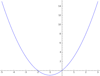
  f(x) = x^2 + 2x 

and graph the function near the point P(2,8).  In the large, the graph y=f(x) of our function should be a parabola.

Zoom in on the point $P(2,8)$ and eventually the graph of the parabola begins to look like a straight line.

If we test a few points, for example (2,8) and (2.1, 8.61), we see that this line has slope about 6.  So the"slope" of the curve y=x^2+2x at the point (2,8) is "about 6."  If the slope of a curve near (2,8) is about 6, then the curve looks like the line y=6x-4.  So the function g(x) = 6x-4 is a good approximation for f(x)=x^2+2x near P(2,8).  Indeed, we could graph both of those functions in the same window of our calculator.

Here (below) we graph the parabola in blue and the line in red.  Notice how closely the line approximates the parabola near the point $P(2,8)$.
(The blue parabola rises just a little above the line at both ends -- it is hard to tell the difference!)

Function slope on a graphing calculator

On a graphing calculator we can often approximate the slope of a function at a point by zooming in on the point until the graph begins to look like a line.  For example, if we wish to find the slope of the curve y=x^2+2x at the point (2,8), we can ask our calculator to graph that curve and then trace the graph until we are on are near the point (2,8).  If we then zoom in on that point, the screen of the calculator should begin to look like the picture below

Or we can create this window directly by setting the window of the calculator as

XMIN = 1.9

XMAX = 2.1

YMIN = 7.4

YMAX = 8.6

To find the slope of this curve, we merely need another point, so the tracing function (on a TI calculator) will give us a point on the curve such as (1.9900, 7.9401).  Once we have this other point, we are ready to compute a slope:

m= (8-7.9401)/(2-1.9900 = (0.0591)/(0.0100 = 5.91.

So the slope of the curve y=x^2+2x at the point P(2,8) is probably about six.

Function notation

A function f on the real line is a mapping from the set of real numbers into the set of real numbers such that each input has a unique output.
It is traditional to use x to label the inputs and y to label the output and write y=f(x) to indicate that y is the result of plugging in x to the function f.  (We do not have to follow this tradition; we will, from time to time, use other letters to indicate inputs to a function or the output of a function.)

Our textbook by Rogawski reviews functions in section 1.1.  Another good source for function review is the online notes by Dr. Paul Dawkins, available here.

The linearization of a function at a point

We seek to replace the function f(x) near a point P(x0, y0) by a straight line, that is, by a linear function L(x) = mx+b where L(x) closely approximates $f(x)$ near $P.$

If we know the slope of the function f(x) at P this is easy to do.   We simply write out the equation for the line through P(x0,y0) with that slope.

For example, consider this problem from my notes:

This problem really just asks for the point-slope form of a line.  Here is the solution.

We will use the point-slope form of a line throughout this class!

Here is a follow-up question (also from my lecture notes)

 The question really relies on the previous work....  The line tangent to the curve at (4,2) has slope 1/8 so it has equation:

y-2 = (1/8)(x-4)

Plug in x=5 to get 

y-2=(1/8)(5-4)=1/8

so

y = 2 + 1/8 = 2.125.

In our Lecture 1.2 (on Friday) we will look at rates of change, both the average rate of change (ARC) and the instantaneous rate of change (IRC).

Week #1 in MATH 1420

For students in the online class at Sam Houston, here is a guide to the expectations for this coming week.

Monday, Jan 16

Although the university is not yet in session, this might be a good time to read through the class syllabus and begin the review worksheet. These materials are on Blackboard and also here in my Google Drive calculus folder.

Tuesday, Jan 17

Complete Worksheet 1.0.  Yes, it is review and extra-credit!  Worksheet 1.0 is in the lecture notes here on Google Drive in Part 1, The Concept of the Derivative. The solutions to odd-numbered problems are here.

Please make sure that your solutions to the homework are written out carefully on your own notebook paper, with lots of room for good mathematical style, function notation, equal signs!

Wednesday, Jan 18

(1) If you intend to submit Worksheet 1.0 for a grade, it should be submitted by 3 pm.

(2) Read Lecture Notes 1.1, available on Blackboard and Google Drive.

(3) Begin Worksheet 1.1. Worksheet 1.1 is in the lecture notes here on Google Drive in Part 1, The Concept of the Derivative. The solutions to odd-numbered problems are here.

(4) Answer the trivia question posed!  There will usually be two questions each week. Solutions MUST be submitted by email to me....

Thursday, Jan 19

Any last questions on Worksheet 1.1? 

Friday, Jan 20

(1) Submit Worksheet 1.1 by 3 pm.

(2) Read Lecture Notes 1.2, available on Blackboard and Google Drive.

(3) Begin Worksheet 1.2. Worksheet 1.2 is in the lecture notes here on Google Drive in Part 1, The Concept of the Derivative. The solutions to odd-numbered problems are here.

Saturday/Sunday, Jan 21-22

(1) Complete Worksheet 1.2 and submit it by 3 pm Monday.

(2) Prepare for to take Mini-exam 1 on Monday.  Mini-exam 1 is over the syllabus, along with Lecture Notes 1.0 & 1.1 & 1.2.

Monday, Jan 23

(1) Take Mini-exam 1 in LDB 207 at 3 pm (unless alternate arrangements have been made.)  

Mini-exam 1 is over the syllabus, along with Lecture Notes 1.0 & 1.1 & 1.2.

(2) Submit Worksheet 1.2 by 3 pm.

More details will be provided on this blog as we go through the week.

Welcome to MATH 1420, a First Course in Calculus!

Next week we start an online class in Calculus 1 at Sam Houston.  As I teach that class, I will also keep a regular blog on the course topics, providing guidance to the lecture notes and homework.

Calculus on Google Drive

In addition to class materials posted on Blackboard, I also maintain a Google Drive folder with class material.  This material, sometimes a little outdated, is available to the public.  It contains past lecture notes, video podcasts, worksheets and worksheet solutions.

Go to this link for my Google Drive calculus folder.

I also maintain a precalculus folder with lots of prerequisite material.  That is available here.