Monday, January 22, 2018

1.2, The ARC and IRC

From the previous section we see that the first step to finding the linearization of a function at a point is the find the slope of the function there.  How do we do that?

Delta f, the slope, and the ARC of a function

Suppose we have a function  y = f(x)  and two points P(x,f(x)) and Q(x+h, f(x+h)).  What is the slope of the line connecting these two points?

The slope of a line connecting P and Q is the difference of y-values divided by the difference of x-values, that is,
m = (f(x+h) - f(x))/(x+h - x).
We may simplify the denominator and write
m = (f(x+h) - f(x))/(h).

Phrased in slightly different notation, the average rate of change (ARC) of a function describes how it changes across an interval from  x1 to  x2.   We compute the change in the function value:
Delta y := y2-y1
 which is the same as  f(x2)-f(x1)  and divide it by the change in  xDelta x := x2–x1.  So the ARC is

ARC := (Delta y)/(Delta x) = (f(x2)-f(x1))/(x2-x1)

There is other notation:  if our first point if P(x, f(x)), (for a particular x value) then we might write our second point as Q(x+h, f(x+h)).   In this case, the ARC is

ARC :=  (Delta y)/(Delta x)  = (f(x+h)-f(x))/h.

Note that the ARC is a slope.  It is the slope of the secant line connecting the two points
 (x, f(x)) and (x+h, f(x+h)).

The Instantaneous Rate of Change

We are really after the instantaneous rate of change (IRC) of a function f(x) at a point  P(x0,f(x0)). The IRC of a function at a point is the slope of the tangent line at that point.

We are really interested in the IRC, not the ARC!  But we only know one point on the tangent line so we cannot directly compute the slope of the tangent line.

Instead we view the tangent line as a limit of secant lines as the point Q gets closer to the point P.
This means that we can estimate the IRC by computing the ARC where the second point Q is very close to the point P.

We can make this precise by introducing the idea of limits, in the next lecture.

Homework over this material

Do Worksheet 1.2 on the ARC & IRC. That worksheet, along with video podcasts on this material, is available here.

Continue reading in Section 2.1 of the Open Stax textbook.

In Spring 2018, Homework 1.2 consisted of the following from the Larson & Edwards textbook: 
HW 1.2 (ARC, IRC and limits)
LE 2.1, p 67: 6-10
LE 2.2, p 75: 1-6, 17-28,

Tuesday, January 16, 2018

1.1, The Slope of a Function

In this lecture we look at the meaning of function slope (with a few examples) and the use of function slope, if it is given to us.  Because of the importance of slope, the most important equation for a line is the point-slope form.

In Spring 2018, the assigned homework from this first lecture is
LE 1.2, p 16: 1-4, 17-22 (put your answer in point-slope form!), 63-66, 76-77,
LE Chap 1 review. p 56: 31-33,
LE 2.1, p 67: 1-5,
And also do the following:
KWS 1.1.1. Assume that the following functions are linear. Linearize the functions (point-slope form!) and then answer the questions.
(a) A function f with slope 30, f(googol) = gazillion. What is f(googol+1)? f(googol+2)? f(googol-1)?
(b) The square root function has slope 1/8 at (4,2). Estimate the square root of 4.1? 4.2? 3.9?
(c) The cube root function has slope 1/12 at (8,2). Estimate the cube root of 8.1? 8.2? 7.9?

A simple idea

The study of science requires an analysis of a variety of functions.  A simple idea with deep and profound consequences is to attempt to treat functions as if, within a short interval, the functions were linear.   Given a particular point P(x, f(x)) on the graph of the function, we ask, "What is the slope of the function at that point?"  In what direction is the function going at that point; how is the function value changing as x changes?

This is an ancient question; its answer has powerful applications.  We will explore the applications first and then develop the tools to find the "slope" of a function.

The slope of a function

The concept of slope (the ratio of the change in output to the change in input) is constant for linear functions and we attempt to generalize that concept to all functions.

For example, take the function
  f(x) = x^2 + 2x 
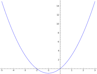
and graph the function near the point P(2,8).  In the large, the graph y=f(x) of our function should be a parabola.


Zoom in on the point $P(2,8)$ and eventually the graph of the parabola begins to look like a straight line.


If we test a few points, for example (2,8) and (2.1, 8.61), we see that this line has slope about 6.  So the"slope" of the curve y=x^2+2x at the point (2,8) is "about 6."  If the slope of a curve near (2,8) is about 6, then the curve looks like the line y=6x-4.  So the function g(x) = 6x-4 is a good approximation for f(x)=x^2+2x near P(2,8).  Indeed, we could graph both of those functions in the same window of our calculator.

Here (below) we graph the parabola in blue and the line in red.  Notice how closely the line approximates the parabola near the point $P(2,8)$.
(The blue parabola rises just a little above the line at both ends -- it is hard to tell the difference!)

Function slope on a graphing calculator

On a graphing calculator we can often approximate the slope of a function at a point by zooming in on the point until the graph begins to look like a line.  For example, if we wish to find the slope of the curve y=x^2+2x at the point (2,8), we can ask our calculator to graph that curve and then trace the graph until we are on are near the point (2,8).  If we then zoom in on that point, the screen of the calculator should begin to look like the picture below

Or we can create this window directly by setting the window of the calculator as
XMIN = 1.9
XMAX = 2.1
YMIN = 7.4
YMAX = 8.6
To find the slope of this curve, we merely need another point, so the tracing function (on a TI calculator) will give us a point on the curve such as (1.9900, 7.9401).  Once we have this other point, we are ready to compute a slope:
m= (8-7.9401)/(2-1.9900 = (0.0591)/(0.0100 = 5.91.
So the slope of the curve y=x^2+2x at the point P(2,8) is probably about six.

Function notation

A function f on the real line is a mapping from the set of real numbers into the set of real numbers such that each input has a unique output.
It is traditional to use x to label the inputs and y to label the output and write y=f(x) to indicate that y is the result of plugging in x to the function f.  (We do not have to follow this tradition; we will, from time to time, use other letters to indicate inputs to a function or the output of a function.)

Our textbook by Rogawski reviews functions in section 1.1.  Another good source for function review is the online notes by Dr. Paul Dawkins, available here.

The linearization of a function at a point

We seek to replace the function f(x) near a point P(x0, y0) by a straight line, that is, by a linear function L(x) = mx+b where L(x) closely approximates $f(x)$ near $P.$

If we know the slope of the function f(x) at P this is easy to do.   We simply write out the equation for the line through P(x0,y0) with that slope.

For example, consider this problem from my notes:


This problem really just asks for the point-slope form of a line.  Here is the solution.

We will use the point-slope form of a line throughout this class!

Here is a follow-up question (also from my lecture notes)


 The question really relies on the previous work....  The line tangent to the curve at (4,2) has slope 1/8 so it has equation:
y-2 = (1/8)(x-4)
Plug in x=5 to get 
y-2=(1/8)(5-4)=1/8
so
y = 2 + 1/8 = 2.125.

In our Lecture 1.2 (on Friday) we will look at rates of change, both the average rate of change (ARC) and the instantaneous rate of change (IRC).

Week #1 in MATH 1420 (Spring 2018)

For students in the spring class at Sam Houston, here is a guide to the expectations for this coming week.

Tuesday, Jan 16
Although the university is not yet in session, this might be a good time to read through the class syllabus and begin the review worksheet. These materials are on Blackboard and also here in my Google Drive calculus folder.

Wednesday, Jan 17
(1) Read Lecture Notes 1.1, available on Blackboard and Google Drive.
(2) Attend class, bringing your textbook and a spiral binder to take notes.
(3) Begin the assigned homework: 

Thursday, Jan 18
Make sure you have a textbook and complete the homework!

Friday, Jan 19
(1) Submit your homework at the beginning of class.
(2) Attend class, bringing your textbook and a spiral binder to take notes.
(3) Begin the assigned homework:

Saturday/Sunday, Jan 20-21
Complete the homework for Monday.

Monday, Jan 22
(1) Submit your homework at the beginning of class.
(2) Attend class, bringing your textbook and a spiral binder to take notes.
(3) Begin the assigned homework:


More details will be provided on this blog as we go through the week.

Welcome to MATH 1420

This week we start a class in Calculus 1 at Sam Houston.  As I teach that class, I will also keep a regular blog on the course topics, providing guidance to the lecture notes and homework.

Calculus on Google Drive

In addition to class materials posted on Blackboard, I also maintain a Google Drive folder with class material.  This material, sometimes a little outdated, is available to the public.  It contains past lecture notes, video podcasts, worksheets and worksheet solutions.

Go to this link for my Google Drive calculus folder.

I also maintain a precalculus folder with lots of prerequisite material.  That is available here.

Monday, May 1, 2017

Week #15 (Last week!) in MATH 1420

Here is a guide to events and assignments in the coming week. This is the last week of the regular semester and we concentrate primarily on reviewing the course.

Monday, May 1, 2017

  1. A trivia question will be posted on Blackboard.
  2. Take Mini-exam 11.  Mini-exam 11 is over lectures 4.1-4.7.
  3. Finish Worksheet 4.7 on integration by substitution.

Tuesday, May 2, 2017

  1. Begin reviewing for the final exam.  Review Parts 1 and 2.
  2. Redo your worst mini-exam from Parts 1 & 2! (You may submit this for up to 10 points extra-credit at the beginning of the final exam.)

Wednesday, May 3, 2017

  1. Worksheet 4.7 is due by 3 pm.
  2. Continue to Review Parts 1 & 2.

Thursday, May 4, 2017

  1. A trivia question will be posted on Blackboard.
  2. Review Parts 3 & 4 for the final exam.
  3. Redo your worst mini-exam from Parts 3 & 4! (You may submit this for up to 10 points extra-credit at the beginning of the final exam.)

Friday, May 5, 2017 

  1. Continue to Review Parts 3 & 4.  
  2. Update any class discussion or online resources on Blackboard.
  3. Make sure you have scheduled your final exam. (Default setting is Monday, 3:30-5:30 pm in LDB 424.)

Saturday-Sunday, May 6-7, 2017

  1. Look for good online videos on calculus. Post a link, with a short review, on Blackboard for any good videos you find.  Then lightly review for the final exam and make sure you get a good night's sleep beforehand!

Sunday, April 23, 2017

Week #14 in MATH 1420

Here is a guide to events and assignments in the coming week.

Monday, April 24, 2017

  1. A trivia question will be posted on Blackboard.
  2. Take Mini-exam 10.  Mini-exam 10 is over lectures 4.1-4.4.
  3. Begin Worksheet 4.5 on the Fundamental Theorem of Calculus.

Tuesday, April 25, 2017

  1. Read OpenStax section 5.3.
  2. Finish Worksheet 4.5.

Wednesday, April 26, 2017

  1. Worksheet 4.5 is due by 3 pm.
  2. Read/watch Lecture 4.6 on the Integral as Net Change
  3. Begin Worksheet 4.6.  It is due on Friday, April 21 at 3 pm.

Thursday, April 27, 2017

  1. A trivia question will be posted on Blackboard.
  2. Read OpenStax section 5.4.
  3. Finish Worksheet 4.6.

Friday, April 28, 2017 

  1. Worksheet 4.6 is due by 3 pm.
  2. Read/watch Lecture 4.7 on the technique of substitution.
  3. Begin Worksheet 4.7.  It is due on Monday, May 1 at 3 pm.

Saturday-Sunday, April 29-30, 2017

  1. Finish Worksheet 4.7.
  2. Read OpenStax section 5.5.
  3. Monday's Mini-exam 11 is over lectures 4.1-4.7.

Friday, April 14, 2017

Week #13 in MATH 1420

Here is a guide to events and assignments in the coming week.

Exam 3 on Monday is over all of chapter 3.

Monday, April 17, 2017

  1. A trivia question will be posted on Blackboard.
  2. Take Exam 3.
  3. Begin Worksheet 4.2.

Tuesday, April 18, 2017

  1. Begin reading in OpenStax chapter 5.
  2. Finish Worksheet 4.2.

Wednesday, April 19, 2017

  1. Worksheet 4.2 is due by 3 pm.
  2. Read/watch Lecture 4.3 on Riemann Sums.
  3. Begin Worksheet 4.3.  It is due on Friday, April 21 at 3 pm.

Thursday, April 20, 2017

  1. A trivia question will be posted on Blackboard.
  2. Finish Worksheet 4.3.

Friday, April 21, 2017 

  1. Worksheet 4.3 is due by 3 pm.
  2. Read/watch Lecture 4.4 on The Derivative of the Signed Area Function.
  3. Begin Worksheet 4.4.  It is due on Monday, April 24 at 3 pm.

Saturday-Sunday, April 22-23, 2017

  1. Finish Worksheet 4.4.
  2. Review OpenStax chapter 5.
  3. Monday's Mini-exam 10 is over lectures 4.1-4.4.